Top Data Analytics terms are explained in this article. Learn these to develop competency in Business Analytics. This will also help you in preparing for the IIBA CBDA Certification.
Data Analytics Terms & Analytics Fundamentals
A
Algorithm
An algorithm is a set of instructions we give a computer in order to take values and manipulate them into a usable form.So, This can be as easy as splitting name and surname with space or as complex as building an equation to predict customer churn in the next quarter.
C
Classification Model
A classification model distinguishes among two or more discrete values or separates data into different classes, like whether an email is a spam or not, will the customer pay his loan on time or not.
Completeness
for instance, Completeness is a data quality dimension and measures the existence of require data attributes in the source in data analytics terms, checks that the data includes what is expected and nothing is missing. For example, the unique record identifier key is not null, or other mandatory fields are not null.
Conformity
Conformity is a data quality dimension, and so it measures how well the data aligns to internal, external, or industry-wide standards. For example, invalid Aadhar card numbers, inconsistent date formats, or violation of allowable values.
Consistency
Consistency is a data quality dimension and tells us how reliable the data is in data analytics terms. So, It confirms that data values, formats, and definitions are similar in all the data sources. For example, telephone numbers with commas in one source and hyphens in another, US and European date formats, and dot and comma decimal separators.
D
Dashboard
A dashboard is a collection of multiple visualizations in data analytics terms that provide an overall picture of the analysis. It combines high performance and ease of use in order to let end users derive insights based on their requirements. They may be interactive, providing insights at multiple levels. For example, some users might prefer sales information at the state level, while some may want to drill down to individual store sales details. Also, see data visualization.
Data Analytics
Data analytics is the science of examining raw data in order to determine valuable insights and draw conclusions for creating better business outcomes. For example, developing proactive campaigns to retain customers.
Data Cleaning
Data cleaning also referred to as data scrubbing or data cleansing and is one of the parts of data analytics terms, is the process of fixing or removing incorrect, corrupted, incorrectly formatted, missing, duplicate, or incomplete data and handling outliers within a dataset. When combining data from multiple data sources, many times, data can be duplicated or mislabeled. For example, correcting spelling mistakes, analyzing customers after a specific date, removing customers before that date will be more meaningful, or fixing structural errors like “Male,” “M” to a similar format.
Data Modeling
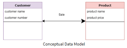
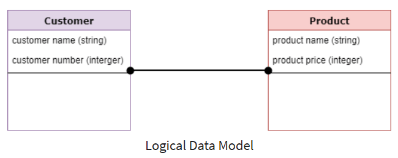
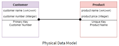
Data modeling is a process used in order to define and analyze data requirements that needs to support the business processes within the scope of corresponding information systems in organizations.
Conceptual Data Model (CDM): Independent of any solution or technology, represents how the business perceives its information.
Logical Data Model: It is an abstraction of CDM. hence, It defines the generic structure of data elements, sets relationships between them, and normalization details.
Physical Data Model: SMEs use it in order to describe how a database is physically organized. So, It represents a database-specific implementation of the data model and helps visualize database structure by replicating database columns, keys, constraints, indexes, triggers, and relationships showing cardinality and nullability.
Useful Links – Data Analytics Certification Training | Data Analytics Fundamentals Course | CBDA certification training | Power BI Certification Course
Data Profiling
In data analytics terms, data profiling establishes data’s profile by determining its characteristics, relationships, and patterns within the data in order to produce a clearer view of its content and quality. So, It involves collecting descriptive statistics, data types, length, and recurring patterns, tagging data with keywords, descriptions, or categories, data quality assessment, risk of performing joins on the data, discovering meta-data, and assessing its accuracy, identifying distributions, key candidates, foreign-key candidates, functional dependencies, embedded value dependencies, and performing inter-table analysis.
Data Validation
Data validation involves checking the accuracy and quality of source data before using, importing, or processing data. While moving or merging data, it is essential that data from different sources is not corrupted and is accurate, complete, and consistent.
Data Visualization
Data visualization is a graphical representation of data in order to determine trends, insights, and complex relationships between variables. Different elements like graphs, charts, and maps help in understanding patterns, trends, and outliers.
Descriptive Analytics
Descriptive analytics provides insight into the past by describing or summarizing data. It aims to answer the question, “What has happened?” For example, aggregating profits across categories and stores.
Diagnostic Analytics
Diagnostic analytics explores why an outcome occurred. It is used to answer the question, “Why did a certain event occur?” For example, investigation of dipping revenue in a particular quarter.
E
Exploratory Data Analysis
Exploratory data analysis is an approach used in data analytics terms in order to maximize the insights gained from data by investigating, analyzing, and summarizing data to uncover relevant patterns using visuals. So, It involves checking consistency and integrity of data, verifying the data dimensions, reviewing descriptive statistics for individual variables, verifying variable inter-dependence and collinearity, formulating missing data, outlier treatment, and data imputation, providing appropriate visualization at relevant steps and deriving preliminary insights, conducting feature engineering, build and test a primary hypothesis to test insights, refine research problems based on insights, report the initial finding with visual analysis.
I
Imputing
Imputing is the process of replacing null or blank values in the data set with meaningful values like mean, median, previous, next value, most frequent, etc., for accurate analysis.
M
Machine Learning
Machine Learning is a branch of artificial intelligence based on the idea that systems/models can learn from data, identify patterns, and make decisions with minimal human intervention.
Metadata
Metadata is the data about data; it gives information about the data. For example, a database will store information about the tables like table name, columns, data types, and descriptions. This is data about the data, i.e., tables in the database.
N
Neural Networks
Neural Networks are algorithms that can recognize underlying relationships in a data set by mimicking how the human brain operates.
O
Online Analytical Processing (OLAP)
An Online analytical processing is software for performing multidimensional analysis at high speeds on large volumes of data from a data warehouse, data mart, or centralized data store.
Online Transaction Processing (OLTP)
An Online analytical processing is another part of data analytics terms that enables the real-time execution of large numbers of database transactions by large numbers of people, typically over the internet. A transaction either succeeds or fails; it cannot remain pending. For example, accurate data processing for ATMs or online banking.
P
Predictive Analytics
Predictive Analytics analyzes past trends in data to provide future insights. It is used to answer the question, “What is likely to happen?” For example: Predicting profit or loss that is likely to happen in the next financial year.
Prescriptive Analytics
Prescriptive Analytics uses the findings from different analytics forms to understand the “what” and “why” of potential future outcomes in data analytics terms. It aims to answer the question “What should happen if we do …?” For example, What will happen to the total sales if the organization adapts the new marketing strategy designed on customer segmentation?
R
Regression Analysis
The Regression analysis is a set of statistical processes for estimating the relationships between a dependent variable and one or more independent variables.
Regression Model
The regression model predicts continuous values like the price of houses, probability of winning.
S
Structured Data
Structured data is organized in tabular form and neatly formatted data, making it easy to store, process, and access excel files, databases, etc.
T
Timeliness
Timeliness is a data quality dimension that tells us whether data is fresh and current and whether data is functionally available when needed.For example, data files are delivered late, updates of scores are not completed on time.
U
Uniqueness
Uniqueness is a data quality dimension that refers to the singularity of records or attributes. For example, identifying any duplicates in the data sets.
Unstructured Data
Unstructured data is not arranged in any order. Irregularities and disorganization make it challenging to handle and work, making it more complex than structured data. It also requires more storage. But it gives more freedom for analysis. Text data, social media comments, documents, phone call transcriptions, various log files like server logs, sensor logs, image, audio, video are examples of unstructured data.

Useful Links – Data Analytics Certification Training | Data Analytics Fundamentals Course | CBDA certification training | Power BI Certification Course
Statistical Tools
A
ANOVA
A statistical analysis method, also known as variance analysis, compares two or more means of samples with a single test and is used in data analytics terms. The independent variables are usually nominal, and the dependent variable is usually interval. The test determines whether the mean differences between these groups are statistically significant.
For example, “What is the difference in average pain level (dependent, interval) among post-surgical patients given three different painkillers (independent & nominal)?” You can determine whether the differences between pain level means for three painkillers are statistically significant.
Null hypothesis: All pairs of samples are the same, i.e., all sample means are equal. Alternate hypothesis: At least one pair of samples is significantly different. The statistics used to measure the significance, in this case, are called F-statistics. Also, see Hypothesis Testing, Nominal Variable, Interval Variable, Sample.
C
Causation
Causation means that one event causes another event to occur. A Causation can only be determined from an appropriately designed experiment. In such experiments, similar groups receive different treatments, and the outcomes of each group are studied. We can only conclude that treatment causes an effect if the groups have noticeably different outcomes. It is also referred to as cause and effect. Also, see Correlation.
Chi-square test
The Chi-square test is used to see if there is a relationship between two categorical variables without assuming cause-and-effect relationships. E.g., How is sports membership related to drama membership in high school students?
Null Hypothesis: Variable A and Variable B are independent.
Alternate Hypothesis: Variable A and Variable B are not independent.
The statistic used to measure significance, in this case, is called the chi-square statistic. It is mainly used to test the significance of statistical independence or association between two or more nominal or ordinal variables.
Confidence Interval and Level
We usually do not have access to the entire population’s values. We can use the sample data to construct a confidence interval to estimate the population parameter with a certain level of confidence. This is a type of statistical inference.
A confidence interval is a range of values derived from sample statistics in data analytics terms, which is likely to contain the value of an unknown population parameter (mean, standard deviation, regression coefficients). If a random sample is drawn multiple times, a certain percentage of the confidence intervals will contain the unknown population parameter. This percentage is the confidence level. Thus, confidence intervals contain a range of reasonable estimates of the population parameter.
For example, to estimate the average happiness score of people between ages 30 to 50, we will have to select a sample as we cannot include the entire population. If we construct a 95% confidence interval for the mean happiness score in the sample. If the 95% confidence interval for the mean is 48 to 52, then it can be said that we are 95% confident that the mean happiness score of all people aged between 30 and 50 is between 48 and 52.
Also, see Population, Sample.
Confounding Variable
A confounding variable is an extra independent variable in analytics that has a hidden effect on the dependent variables. They are closely related to the independent and dependent variables.
For example, the sales for chocolates and cookies increased in parallel with a retail store’s operational costs in July and August. Does this mean that an increase in cookies and chocolates causes an increase in operational costs? That is not the case. The holiday season is the confounding variable bringing both the factors (increase in sales and operational costs) together.
Also, see Causation and Correlation.
Continuous Variables
Continuous variables have an infinite range of possible values. Contrast to discrete variables.
For example, time, or temperature, can take on a value between any other two values like 15.4°C or 15.46°C or 15.467°C.
Correlation
Correlation shows if there is a relationship or pattern between the values of two variables. It measures both the direction (positive or negative or none) and the strength of the linear relationship between two variables (coefficient of correlation with a value between -1: high negative correlation and +1: high positive correlation).
When X is higher, Y also tends to be higher, showing a positive correlation, and when X is higher, Y tends to be lower shows a negative correlation.

For example, Ice-cream sales and temperature will show a moderate negative correlation.
Correlation does not necessarily imply causation. Correlation indicates that the values vary together. It does not necessarily suggest that changes in one variable cause changes in the other variable.
Also, see Causation.
Covariance
Covariance evaluates the extent to which one variable changes in relation to the other variable. We can only get an idea about the direction of the relationship, but it does not indicate the relationship’s strength. A positive covariance denotes a direct relationship, whereas a negative covariance denotes an inverse relationship. The value of covariance lies in the range of -∞ and +∞.
D
Descriptive Statistics
Descriptive statistics are non-parametric statistics that provide simple, quantitative summaries of datasets, usually combined with explanatory graphics. They provide easy-to-understand information that helps answer basic questions based on the average, spread, deviation of values, and so on. They give a rough idea about what the data is indicating so that later they can perform more formal and targeted analyses.
For example, measures of central tendency give a one-number summary of the central point of the dataset, and measures of dispersion describe the spread of the data around the central value.
Discrete Variable
A discrete variable is measured only in whole units like the number of players, the number of participants, or the count of model products.
Distribution
Distribution is the arrangement of data by the values of one variable, from low to high. This arrangement, and its characteristics, such as shape and spread, provide information about the underlying sample.
E
Error
Error is the difference between the actual and the predicted value. (Actual value – Predicted value).
Error Rate
The inaccuracy of predicted output values is termed the error of the model. The error rate is used to assess the model performance of how often the model predicts incorrectly. It can be calculated as (FP+FN)/(TP+FP+TN+FN).
H
Hypothesis Tests
Hypothesis tests are also called significance tests in data analytics terms. A hypothesis test starts with some idea of what the population is like and then tests to see if the sample supports this idea. They are used mainly in problem analysis to transform intuitive assessments into verifiable and measurable evaluations or a research problem. It provides a scientific way to verify hunches, intuition, and experience-based decisions.
It is advantageous when data captured is limited to only a subset or sample of the whole population. Every hypothesis test contains two hypotheses – the null and the alternative hypotheses. Typically, the null hypothesis says that nothing new is happening and is denoted as H0. In general, we assume the claim to be valid until proven otherwise. The alternate hypothesis is the negation of the default position. It is denoted as H1.
For example,
Null hypothesis = “no difference between the means of group A and group B”;
Alternative hypothesis = “A is different from B” (could be bigger or smaller)
I
Inferential Statistics
Inferential Statistics helps draw inferences and generalizations for the population by assessing the sample subset.
For example, the population can comprise all customers using the mobile network of a company ABC across geographies. It is not possible many times to survey the entire population given the large number; hence, we select a smaller group from the population. It is representative of the population. Inferential statistics include hypothesis testing, regression analysis, and Bayesian inference.
Also, see Hypothesis Testing, Regression Analysis.
Interquartile range (IQR)
The interquartile range is the difference between the upper (Q3) and lower (Q1) quartiles. It is less sensitive to extreme outliers than the range as a measure of the spread of data.

Also, see Outliers, Range.
Interval Variable
An interval variable is a variable in which both order of data points and the distance between them can be determine, but it has no real zero-point like temperature, pH, and SAT score. In this case, no zero point means that 100°F is not “5 times as hot as” 20°F.
K
Kurtosis
Kurtosis describes whether the data is light-tailed – indicating lack of outliers or heavy-tailed – indicating the presence of outliers compared to a normal distribution. Low kurtosis in a data set is an indicator that data has light tails or lack of outliers. Histogram works well to show kurtosis.
Also, see Outliers, Range.
M
Mean
Mean is the average score within a distribution. It is the ratio of the sum of all values in the data to the total number of values.
Mean Absolute Error
Mean absolute error is one of the many metrics to summarize and assess the machine learning model’s quality. It is the average of the absolute errors in a set of predictions.

Also, see Error.
Mean Squared Error
Mean squared error is the sum of the square of the difference between the predicted and actual value divided by the total number of data points. It measures the variance of the residuals.
Mean Squared Error
Median
Median is the center score in a distribution.
For example, median of 25, 40, 75, 80, 65, 69, 60, 57, 75, 54, 50 is 60.
Mode
Mode is the most frequent/popular score in a distribution.
For example, mode of 25, 40, 75, 80, 65, 69, 60, 57, 75, 54, 50 is 75.
Useful Links – Data Analytics Certification Training | Data Analytics Fundamentals Course | CBDA certification training | Power BI Certification Course
Monte Carlo Simulation
Monte Carlo Simulation is a mathematical problem-solving and risk-assessment technique used in data analytics terms that approximates the probability and risk of specific outcomes using computerized simulations of random variables. It is helpful to understand better the implications of a particular course of action or decision.
For example, telecom companies use this simulation to assess network performance in different scenarios, optimizing the network.
Also, see Probability.
N
Nominal Variable
A nominal variable is a variable determined by categories that cannot be ordered, like gender and color.
Normal Distribution
Normal Distribution is the most common distribution. Here, the mean, median, and mode of the Distribution are equal, and the curve of the Distribution is bell-shaped, unimodal, and symmetrical about the mean. The curve’s spread is determined by its standard deviation (σ), showing that more data is near the mean (μ). The total area under the curve is one as it represents the probability of all outcomes.
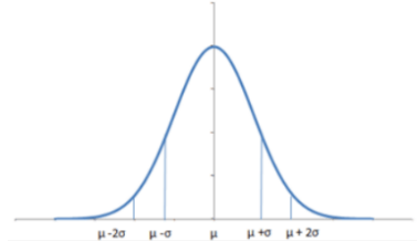
Also, see Mean, Standard Deviation.
O
Ordinal Variable
An ordinal variable is a variable in which the order of data points can determine but not the distance between them.
For example, socioeconomic status (“low,” “medium,” “high”), income level (“less than 50K”, “50K-100K, “over 100K”), question type (very hard/somewhat hard/okay/easy/very easy).
Outliers
Outliers are values that are distant from most other values.
P
P-Value
P-value tells us that if the p-value(probability) is less, then the null hypothesis does not hold in real life. If the p-value is lower than a predetermine significance level(alpha), usually 0.05, then the null hypothesis is rejected.
For example, if the pizza delivery time is 30 minutes or less (null hypothesis is true), how true is it in real life? This is answered by p-value probability. If we find that the mean delivery time is longer by 10 mins and we get the p-value as 0.03, there is a 3% chance that the mean delivery time is at least 10 minutes longer due to noise. As this p-value is less than alpha (0.05), the null hypothesis of a mean delivery time of fewer than 30 minutes is rejected.
Also, see Hypothesis Testing.
Percentile
Percentiles split the sample data into hundredths. Percentiles indicate the values below which a certain percentage of the data in a data set is found. They help understand where a value falls within a distribution of values, divide the dataset into portions, identify the central tendency, and measure a distribution’s dispersion.
The 25th percentile is equivalent to the lower quartile, and the 50th percentile is the same as the median.
For example, the score of a batch of students is as follows: 25, 40, 50, 54, 57, 60, 64, 65, 69, 75, 75, 76, 80, 80, 84. The 3rd value is 50, which marks the 20th percentile of the students in the class. This indicates that 20% of students earned a score of 50 or lower.
Population
The population is the target group under investigation, like all working people earning a daily salary. The population is the entire set under consideration. Samples are drawn from populations.
Also, see Sample.
Probability
Probability is the chance that a phenomenon has of occurring randomly.
R
Range
The range is the difference between the highest and lowest scores in a distribution. For example, range of 25, 40, 75, 80, 65, 69, 60, 57, 75, 54, 50 is 80 – 25 = 55
It describes only the data’s width but not how it is dispersed between the range. It is sensitive to outliers and may give misleading results in that case.
Ratio Variable
A ratio variable is a variable in which both order of data points and distance between them can be determine, and for which there is a real zero point, such as weight or distance.
Residual
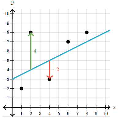
A residual is a measure of how well a line fits an individual data point.
It is the vertical distance between a data point and the regression line. If the data point is above the regression line, it is positive; if the data point is below the regression line, it is negative, and if the regression line passes through the point, it is zero.
Root Mean Squared Error
Root mean squared error is the square root of the average of squared differences between prediction and actual observation. (The square root of mean squared error.)
Also, see Mean Squared Error.
S
Sample
It is not possible many times to survey the entire population given the large number; hence, a smaller group is selected. This sample is representative of the population. By studying the sample, the researcher tries to draw valid conclusions about the population.
Also, see Population.
Skew
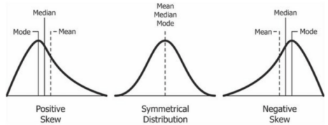
Skew is the measurement of symmetry in a probability distribution. The positions of median, mode and mean for different skewness in data. A histogram is effective in showing skewness.
Skewness gives us an idea about the direction of the outliers and is also used in data analytics terms.
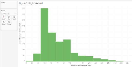
For example, this histogram shows the maximum wind speed of all the hurricanes. We can observe that most of the distribution is saturated on the left side between 30 – 40 Kt. This tells us that the maximum wind speeds are concentrated on the lower side, indicating that not many storms are severe.
Also, see Mean, Median, Mode.
Standard Deviation
Standard deviation is the variance that gives the spread in terms of squared distance from the mean, and the unit of measurement is not the same as the original data.
For example, if the data is in meters, the variance will be in squared meters is not intuitive. It is the square root of variance.
Also, see Variance, Mean.
Standardization (Z-Score normalization)
The independent features will be rescaled to have the properties of a standard normal distribution with a mean of 0 and a standard deviation of 1. They can be calculated using the formula for z scores:

It is useful for comparing measurements that have different units. Also, see Normal Distribution, Mean, Standard Deviation.
Statistics
Statistics is a form of mathematical analysis of data leading to reasonable conclusions from data. It is helpful while evaluating claims, drawing key insights, or making predictions and decisions using data.
T
Test Statistic
A test statistic is a random variable calculated from the sampled data under the assumption that the null hypothesis is correct. The test statistics magnitude becomes too large or too small when the data shows strong evidence against the null hypothesis premises. Different hypothesis or statistical tests like Z-test, t-test, ANOVA, Chi-square test use various test statistics like Z-statistic, t-statistic, f-statistic, and Chi-square statistic respectively.
Also, see Hypothesis Tests.
Useful Links – Data Analytics Certification Training | Data Analytics Fundamentals Course | CBDA certification training | Power BI Certification Course
T-test
The T-test is used to compare the mean of precisely two given samples. (Paired t-test: Samples from the same population, Independent t-tests: Samples from different populations.) Like a z-test, a t-test also assumes a normal distribution of the sample. A t-test uses when the population parameters (mean and standard deviation) are not known. The statistic for this hypothesis testing is called t-statistic. Also, see z-test.
Also, see Mean, Population, Hypothesis Tests.
V
Variance
Variance is the variability of model prediction for a given data point. A model with high variance pays a lot of attention to training data and does not generalize on unknown data. Hence, such data analytics terms perform very well on training data but have high error rates on test data. Also, see bias.
Variance is also a statistic of measuring spread, and it is the average of the distance of values from the mean squared.

Z
Z-Test
The sample is assumed to be normally distributed. A z-score is calculate with population parameters such as “population mean” and “population standard deviation” and is use to validate a hypothesis that the sample drawn belongs to the same population.
Null hypothesis: Sample mean is the same as the population means.
Alternate hypothesis: Sample mean is not the same as the population mean.
The statistics used for this hypothesis testing are called z-statistic. Also, see Mean, Population, Hypothesis Tests.
You can also explore our more blogs related to Exploratory Data Analysis, Structured & Unstructured Data, Extract Transform Load, and many more…
Data Workflow Elements
The Data workflow elements are as follows:
Data Governance
A Data governance involves processes and practices which enable formal and proper management of data assets in an organization. It deals with security, privacy, integrity, usability, integration, compliance, availability, roles, responsibilities, and management of its internal and external data flows.
Data Mart
Datamart is a subset of a data warehouse focused on a particular line of business, department, or subject area. It provides quick access to specific data to a defined group of users to access critical insights without searching the entire warehouse.
For example, a data mart may be align with a specific business department, such as finance, sales, or marketing.
Data Migration
Data migration refers to transferring data from one system to another while changing the storage, database, or application. It usually happens during an upgrade of existing hardware or transfers to an entirely new system.
Data Mining
Data mining is a subset of business analytics that looks for patterns, associations, correlations, or anomalies existing in large data sets to gain insights or solve business problems.
For example, finding unknown patterns in the data and identifying new associations could indicate customer churn in the future.
Data Lake
The data lake contains aggregated data—independent of format or source, structured and unstructured—into a single repository. Data lakes enable businesses to perform broad data exploration, discovery, and analytics on all available data, resulting in better insights and informed decisions.
Data Vault
The Data Vault is a detail-oriented, history-tracking, and uniquely linked set of normalized tables that support one or more functional areas of business.
Instead of building the entire warehouse, data vaults enable enterprises to start small and build incrementally over time. Changes to business rules can be easily incorporate against a data warehouse. No rework is need when adding additional sources. Raw data is also to include, which helps back-populate the presentation area with historical attributes that were not initially made available.
Data Warehouse
A data warehouse is a collection of structured, integrated, subject-oriented databases designed to supply decision-making information. The data sources connect to the data warehouse through an ETL process.
Also, see Extract Transform Load.
Data Wrangling
Data wrangling, also known as data munging, is one of the first and most essential steps in any data-related project or work. It involves the preparation of data for accurate analysis: data sourcing, profiling, and transformation.
Extract Transform Load
Organizations collect a lot of data stored in varied formats from different sources. Migrating one or more of these data sources into a single data repository, where all data has a consistent format, allows for easy access to the organization’s data and reporting. Extract Transform Load is a data analytics terms, used to make data available from various data sources to a target repository that acts as a single standardized source of truth for further analysis to drive essential insights.
Machine Learning Techniques
A B C D F H L N O P R S T U W
A
Accuracy
Accuracy is used to assess the model performance. It answers the question: “How often does the model predict correctly?” It can be calculated as (TP+TN)/(TP+FP+TN+FN).
Accuracy is also a data quality dimension related to the precision of data.
For example, data records at the wrong level of precision or have not been updated.
Also, see the True Positive, True Negative, False Positive, False Negative.
Area Under the ROC Curve
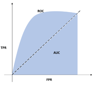
AUC – ROC curve is a performance measurement for the classification problems at various threshold settings. ROC is a probability curve, and AUC represents the degree or measure of separability in data analytics terms. It tells how much the model is capable of distinguishing between classes. Higher the AUC, the better the model is at predicting 0s as 0s and 1s as 1s.
For example, the higher the AUC, the better the model distinguishes between patients with cancer and those without. Also, see Receiver Operator Characteristic Curve.
B
Bias
Bias is the difference between the model prediction and the actual value. A model with high bias pays very little attention to the training data and oversimplifies the model (underfitting). It always leads to a high error on training and test data.
Also, see Underfitting, Variance.
Binary Classification
Binary classification outputs one of the two mutually exclusive classes.
For example, classifying patients with tumors and without tumors, customer churn prediction – yes or no.
Common Machine Learning Algorithms: K-Nearest Neighbors, Decision Trees, Random Forest, Support Vector Machine (SVM), Naive Bayes, Logistic Regression.
C
Clustering
Clustering refers to grouping elements together to separate data points into different categories.
For example, market segmentation: Clustering similar people based on product categories they buy, Customer segmentation: Grouping individuals similar in specific ways relevant to marketing such as age, gender, interests, spending habits, etc.
Common Machine Learning Algorithms: K-Means Clustering, Mean-shift Clustering, Hierarchical Clustering
Confusion Matrix
An NxN table that summarizes how successful a classification model’s predictions are. One axis contains the actual values, and the other has predicted values.
Also, see True Positive, False Positive, True Negative, False Negative.

D
Decision Trees
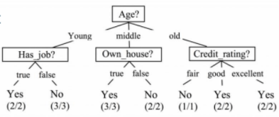
The decision tree model represents a sequence of branching statements and potential outcomes. Each node represents a feature (attribute), each link (branch) represents a decision (rule), and each leaf represents an outcome. They provide a practical structure that lays out options and investigates the possible outcomes of choosing those options.
In machine learning, a decision tree is a supervised machine learning technique primarily used in classification.
Also, see Supervised Machine Learning.
F
False Positive
False Positive is an outcome where the model incorrectly predicts the positive class.
For example, predicting that a person has a tumor, but in reality, the person does not have it. The prediction was positive but wrong.
False Negative
A false negative is an outcome where the model incorrectly predicts the negative class.
For example, predicting that a person does not have a tumor, but in reality, the person does have. The prediction was negative but wrong.
Feature
A feature is an input variable to a model and is used for analysis. In datasets, features appear as columns. Features are also sometimes refer to as “variables” or “attributes.” The features’ quality decides the quality of the insights that gains when the dataset is use for analysis.
For example, features like the number of bedrooms, area, etc., can predict the house price.
Feature Engineering
Feature engineering is the process of creating features from raw data in data analytics terms. It is the addition or construction of additional features which can improve the model performance and accuracy.
For example, creating a profit ratio using profit and sales fields, or scaling, normalizing data, or extracting some specific features from the date as the weekday’s name, etc.
Also, see Feature.
Useful Links – Data Analytics Certification Training | Data Analytics Fundamentals Course | CBDA certification training | Power BI Certification Course
Feature Selection
Feature selection is the process of selecting a subset of relevant features (variables, predictors) for use in machine learning model construction. It does not involve creating new features or transforming existing ones but eliminating the features that do not add value to the analysis.
Also, see Feature.
H
Heteroskedasticity
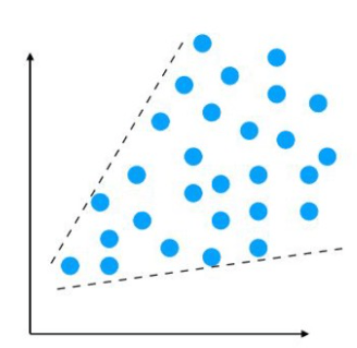
Heteroskedasticity refers to situations where a variable’s variance is unequal across the range of values of the second variable that predicts it. Visually, it displays an unequal scatter seen as a fan or cone on a scatter plot.
For example, if we want to predict income based on age, we will probably see more variability as the age increases.
L
Label
A label is a variable that we predict, like price, prediction of the presence of cancer (yes/no).
N
Normalization
Normalization is the process of converting an actual range of values into a standard range of values, typically -1 to +1 or 0 to 1. It is use to build features with a similar range, making it easier and more accurate for analysis.
For example, if a machine learning model is trying to predict the best house fit for you by looking at the predictors – cost and number of rooms. So, There will be a considerable difference in cost between a house with two rooms and ten rooms; the difference in the number of rooms contributes less to the overall difference. The difference in the number of rooms would be less relevant because the cost of two houses could have a difference of thousands of dollars.
The goal is to make every data point have the same scale, so each feature is equally important. Also, see Feature.
O
Overfitting
Overfitting occurs when a model tries to fit the training data so closely that it does not generalize new data. This model will have to give high accuracy on the training data but low accuracy on new data.
Also, see Training dataset, Accuracy.
P
Precision
Precision is used to assess the model performance to assess that when it predicts yes, how often is it correct? It is calculated as TP/(TP+FP).
For example, when it predicts that a particular person has cancer, how often is it correct? Also, see True Positive, False Positive.
R
Receiver Operator Characteristic Curve
The Receiver Operator Characteristic Curve is a curve of true positive rate vs. false positive rate at different classification thresholds.
Also, see Area Under the ROC Curve.
S
Scaling
Scaling is converting floating-point feature values from their natural range (for example, 1 to 10,000) into a standard range (for example, 0 to 1 or -1 to +1).
Also, see Feature.
Sensitivity/Recall
Sensitivity/Recall is use in order to assess the model performance for the proportion of actual positive cases that predicts as positive. It answers the question. “When it is actually yes, how often does the model predict yes?” It is calculated as TP/(TP + FN).
For example, it will indicate the proportion of sick people and got predicted correctly as being sick. Also, see True Positive, False Negative.
Specificity
Specificity uses in order to assess the model performance for the proportion of actual negative cases that got predict as negative. It answers the question. “When it is actually no, how often does the model predict no?” It is calculated as TN/(FP + TN).
For example, it will indicate the proportion of people who were actually not sick and predicts correctly as not sick. Also, see True Negative, False Positive.
Supervised Machine Learning
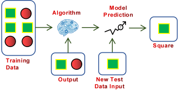
Like observing and learning, supervised machine learning models learn from training data where the input and expected output are known. It iterates predicting, learning, and improving on the training data until an acceptable accuracy is reached. Thus, the model is supervised to learn and achieve higher accuracy. This trained model is then use on the test data to predict the output of new inputs. Classification and Regression come under supervised learning.
Also, see Training Dataset, Test Dataset, Classification Model, Regression Model, Accuracy.
T
Test Dataset
The test dataset is a subset of the original data to test the trained model.
Training Dataset
The training dataset is a subset of the original data to train a model.
True Negative
True negative is an outcome where the model correctly predicts the negative class.
For example, predicting that a person does not have a tumor, and in reality, the person does not have. The prediction was negative and correct.
True Positive
True Positive is an outcome where the model correctly predicts the positive class.
For example, predicting that a person has a tumor, and in reality, the person does have. The prediction was positive and also correct.
U
Underfitting
Underfitting occurs when a model is too simple with too few features, and it cannot capture the underlying trend of the data. Underfitting makes it inflexible in learning from the dataset.
Also, see Feature.
Unsupervised Machine Learning
In unsupervised learning, no output data is available for machines in order to learn. The objective is to look at the input data structure and learn more to try and find patterns. hence, There is no correct answer, and models must work without any guidance from data. Examples are Clustering and Segmentation algorithms.
Also, see Clustering.
W
Weighting
Weighting is a correction technique for uneven representation in which sample weights can apply to address the probability of unequal samples and survey weights are applies in order to address bias in surveys. It helps eliminate bias in a sample dataset.
Also, see Probability, Bias.
About Techcanvass
Techcanvass is an IT training and consulting organization. We are an IIBA Canada Endorsed education provider (EEP) and offer business analysis certification courses for professionals.
We offer Data Analytics Certification Training, Data Analytics Fundamentals Course, and CBDA certification training to help you gain expertise in data analytics terms and work as a Business Analyst in Data Science projects. You can also learn Data visualization skills by joining our Power BI Certification Course.


