Introduction to Descriptive Statistics
Statistics is a form of mathematical analysis of data leading to reasonable conclusions from data. It is useful while evaluating claims, drawing key insights, or making predictions and decisions using data. In this guide, let us understand descriptive statistics in its depth.
We can say that statistics is a crucial field of mathematics, which data scientists use for analyzing, interpreting, and predicting the desirable outcomes from the given data. Moreover, as the name suggests, descriptive statistics will help you understand the statistical concepts to describe various data.
And as we know, descriptive statistical analysis is an essential part of machine learning and is absolutely crucial for any business. Therefore, it is important to understand what descriptive statistics is all about as it is going to help you get clarity on how to identify different types of data.
Types of Data
Data comes in various formats like age, income, sales or profits, and race, gender, name, or address. The data type determines the type of statistics that can be used. Data types can broadly be defined as ‘quantitative’ if it is numerical and ‘qualitative’ if not. Qualitative data can contain unstructured data, like photographs, videos, sound recordings, and so on.
You can read our post related to Structured Vs. Unstructured Data in data analytics and grow your Skills.
https://businessanalyst.techcanvass.com/
Let us look at the different types of data:
Useful Links – CBDA Training
Statistical Distribution
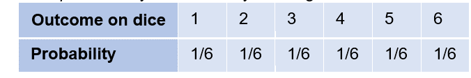
A statistical distribution is a mathematical function that gives the probabilities of all possible outcomes of a random variable. There are discrete and continuous distributions depending on the variable it models. Example: When you roll a die, you can get either 1, 2, 3, 4, 5, or 6. All numbers have an equal chance.
Let us understand some common examples:

Bernoulli distribution (Discrete Distribution): A Bernoulli distribution has only two possible outcomes, namely 1 (success) and 0 (failure), and a single trial.

A normal distribution (Continuous Distribution): This is the most common distribution. Here, the mean, median, and mode of the distribution are equal, and the curve of the distribution is bell-shaped, unimodal, and symmetrical about the mean. The spread of the curve is determined by its standard deviation (σ) showing that more data is near the mean (μ). The total area under the curve is 1, as it represents the probability of all outcomes.
What is Statistical Analysis?
Statistical analysis is the process of collecting, observing, manipulating, summarizing, and interpreting qualitative or quantitative data to identify trends and relationships in the data.
Statistical analysis can be divided into descriptive statistics, which help us understand the data by providing summaries such as percentages, means, variances, and correlations, and inferential statistics, which helps infer properties of the population using t-tests, chi-square tests, regression, and analysis of variance (ANOVA).
What Are Descriptive Statistics?
Descriptive statistics are used for describing a particular dataset. It involves various tasks such as collection, organization, summarization, displaying, and analyzing the data to understand it in its depth and visualize the data for efficient decision making. Descriptive statistics can be categorized into measures of central tendency and measures of variability (spread) or also known as measures of dispersion. These types further include various elements of descriptive statistics.
After a data scientist collects the data, the first step in the statistical analysis process is descriptive statistics that involves using various techniques to describe a dataset. Therefore, one uses descriptive statistics to repurpose hard-to-understand quantitative data. One good example is the student’s grade point average (GPA). The idea behind calculating the GPA is that it considers data points from a wide range of exams, classes, and grades to find the mean academic performance of a student.
Types Of Descriptive Statistics
The different types of descriptive statistics are as follows:
| Measures of Central Tendency | Measures of Variability/Dispersion | Measures of Association |
| Uni-variate Analysis | Uni-variate Analysis | Bivariate and Multivariate Analysis |
| Mean, median, mode | Range, percentiles, quartiles, variance, standard deviation, standard score/z-score, skewness, and kurtosis | Covariance and correlation |
Measures of Central Tendency
These statistics are a one-number summary of the data that typically describes the center of the data. It gives a typical value or the middle of the data. The measures of central tendency have the following types:
Mean
Mean is defined as the ratio of the sum of all the values in the data to the total number of values. It is applicable to numerical variables only. It is the most common method for finding the average. To understand it better, consider the following example.

Suppose, we have a sample of student grades as: 25, 40, 75, 80, 65, 69, 60, 57, 75, 54, 50. The mean can be calculated as 59.09 using the following formula:
M= Sum of all the terms/ Number of terms
Median
Median is the value that divides the data into two equal parts when data is arranged in either ascending or descending order. It applies to numerical variables only. Median is the middle term in a data set.
- It will be the middle term when the number of terms is odd. Median of 25, 40, 75, 80, 65, 69, 60, 57, 75, 54, 50, after arranging in ascending order: 25, 40, 50, 54, 57, 60, 65, 69, 75, 75, 80 is 60.
- It will be the average of the middle two terms when the number of terms is even. Median of 200, 25, 40, 75, 80, 65, 69, 60, 57, 75, 54, 50 after arranging in ascending order: 25, 40, 50, 54, 57, 60, 65, 69, 75, 75, 80, 200 is 62.5 (average of 60 and 65).
Mode (Mo)
The mode of a set of data is the most popular value, the value with the highest frequency. Unlike the mean and median, the mode has to be a value in the data set. It is applicable to numerical as well as categorical variables.
Mode of 25, 40, 75, 80, 65, 69, 60, 57, 75, 54, 50 is 75.
There could be data sets with no repeating values and hence no mode, bimodal data sets with two repeating values, or multimodal data sets with many repeating values.
Measures of Variability/Dispersion
Even if two data sets have the same mean, there may be differences between the data sets. We can differentiate between each data set by looking at the spread of values from the mean. Measures of dispersion describe the spread of the data around the central value.
Measures of variability or measures of dispersion help the data scientist analyze how dispersed the distribution may be for a given dataset. This type of descriptive statistics helps in describing how the data set is distributed within the dataset. It includes the following:
Range
The range is a very easy way of measuring how to spread out the values are. It is the difference between the largest and the smallest data values. Consider the following example:
Range of 25, 40, 75, 80, 65, 69, 60, 57, 75, 54, 50 is 80 – 25 = 55
The formula for the range is- Xmax – Xmin
Percentiles
Percentiles indicate the values below which a certain percentage of the data in a data set is found. They help to understand where a value falls within a distribution of values, divide the dataset into portions, identify the central tendency, and measure the dispersion of a distribution. Median is the 50th percentile.
To calculate percentile, values in the data set should always be in ascending order. The formula is:

where N = number of values in the data set, P = percentile, and n = ordinal rank of a given value in ascending ordered data.
Quartiles
Quartiles are values that divide the data into quarters, and they are based on percentiles. Q2 is the median. The interquartile range (IQR) is a measure of statistical dispersion between upper (75th) and lower (25th) quartiles. There are four quarters that divide the data sets into quartiles, they are as follows:
- Lowest 25% of numbers.
- Next lowest 25% of numbers (up to the median).
- Second highest 25% of numbers (above the median).
- Highest 25% of numbers.
Variance
Range and interquartile range indicate the difference between high and low values, but we don’t get an idea about the variability of the data points. Variance is a statistic of measuring spread, and it is the average of the distance of values from the mean squared.

where N is the total number of data points, Xi is the data values and X̄ is the mean.
The sum of the distance of values from the mean will always be 0, hence we need to square them. A high variance indicates that data points are spread widely in between the range.
Standard Deviation (σ)
The variance gives the spread in terms of squared distance from the mean, and the unit of measurement is not the same as the original data. For example, if the data is in meters, the variance will be in square meters, which is not very intuitive. We take the square root of the squared variance to get the standard deviation (σ).

The smaller the standard deviation, the closer values are to the mean. The smallest value the standard deviation can take is 0.
Standard Scores/ Z-score
Standard scores give you a way of comparing values across different data sets where the mean and standard deviation differ. For example, if you want to compare sales across two different locations having different mean and standard deviations, standard scores would help.
Z-score is measured in terms of standard deviations from the mean and shows how far away the value is from the mean. The formula is:
Useful Links – CBDA Training

Skewness
Skewness is a measurement of symmetry in a probability distribution. You can see the positions of median, mode, and mean for different skewness in data. A histogram is effective in showing skewness.
Data scientists basically use Skewness for understanding the distribution of a given dataset and what steps can be taken for normalizing the data for the further creation of machine learning models.
Pearson Second Coefficient of Skewness (Median(M) skewness) is the most common method of calculating skew. The sign gives the direction of skewness. The larger the value, the larger the distribution differs from a normal distribution. The formula is as follows:

Kurtosis
Kurtosis describes whether the data is light-tailed, indicating lack of outliers, or heavy-tailed, indicating the presence of outliers when compared to a normal distribution. Histogram works well to show kurtosis. There are three types of kurtosis.
- Mesokurtic distributions: Kurtosis is zero, and it is similar to the normal distributions.
- Leptokurtic distributions: The tail of the distribution is heavy, indicating the presence of outliers, and kurtosis is higher than the normal distribution.
- Platykurtic distributions: The tail of the distribution is thin, indicating a lack of outliers, and kurtosis is lesser than the normal distribution.
You may also like our latest blog related to “Data Analytics Lifecycle Phases“, click on the link, and explore other areas of Data Analytics.
Measures of Association
Measures of association quantify a relationship between variables. The mathematical concepts of covariance and correlation are very similar. Both describe the variance between two variables.
Covariance
Covariance evaluates the extent to which one variable changes in relation to the other variable. We can only get an idea about the direction of the relationship but it does not indicate the strength of the relationship.
A positive covariance denotes a direct relationship, whereas a negative covariance denotes an inverse relationship. The value of covariance lies in the range of -∞ and +∞. The magnitude of the covariance is not standardized and hence depends on the magnitudes of the variables. The formula to calculate covariance is:

It helps find essential variables on which other variables depend and predict one variable from another.
Correlation (ρ)
Correlation is an important statistical technique for multivariate analysis that shows how strongly the variables are related. It measures both the direction (positive or negative or none) and the strength of the linear relationship between two variables. It is a function of the covariance and can be obtained by dividing the covariance by the product of the standard deviation of both variables.

The difference between covariance and correlation lies in the values; correlation values are standardized (between -1 and +1). It outputs the correlation coefficient (r), which does not have any dimension, ranging from -1 and +1. Value or r closer to -1 (negative) or +1 (positive) indicates high correlation.
Conclusion
This article gives you an overview of what descriptive statistics is all about and what are its types. Descriptive statistics are broken down into measures of central tendency, measures of variability/dispersion, and measures of association. The in-depth understanding of the types of descriptive statistics will allow you to easily identify the type of data in your work role.
Descriptive statistics is a very important concept in data analytics as it allows us to visualize and interpret the raw data in a more simple and straightforward way. If you are curious to know more about data science as a career, explore various data science courses at Techcanvass.

Frequently Asked Questions (FAQs)
We need statistics to simply describe the data because if we present raw data, then it would become hard for the data scientists to visualize and understand the data. Therefore, we can say that statistics help in visualizing and describing the data in a meaningful manner.
Mean deviation is the statistical measure, which is used for calculating the average deviation from the mean value of a given data set. Standard deviation is also a statistical measure, but it is used to calculate the dispersion of a dataset relative to its mean.
One can use descriptive statistics for summarizing and organizing the data to understand it better. Descriptive statistics does not attempt to make inferences or predictions. However, it can be used along with inferential statistics to make predictions or inferences.
Statistics study the entire data to interpret it and analyze it for meaningful insights and derive successful outcomes.
The most commonly used descriptive statistics are the measures of central tendency-the mean, mode, and median. Measures of central tendency are used at all levels of math and statistics and are the most common.
Descriptive statistics revolves around describing the general characteristics of data and summarizing it. While inferential statistics make predictions or inferences about a larger dataset based on the sample of that data.
Descriptive statistics helps to describe the size, center, spread, and other characteristics of data. The basic purpose of descriptive statistics on a data set is to figure out the basic details about the variables in the dataset or to determine the relationship among variables.